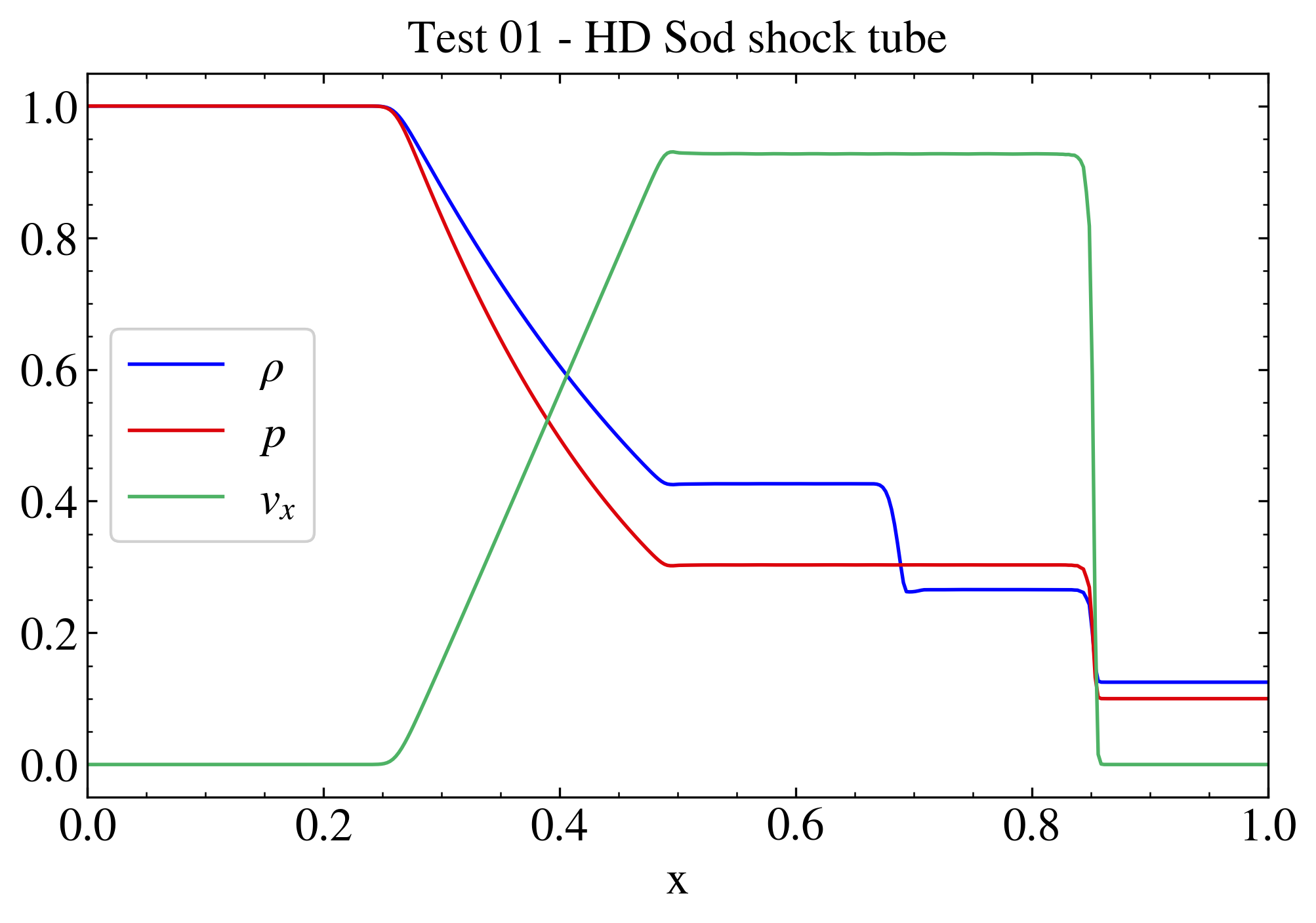
"""HD shock tube test.

This test shows how to plot different 1D quantities from a test problem
in the same plot.

The data are the ones obtained from the PLUTO test problem
$PLUTO_DIR/Test_Problems/HD/Sod (configuration 1).

In this script the plotted variables are density, pressure and velocity
(component x) in different colors. The relevant keywords to customize
the plot (e.g., the labels or the legend position) are scattered through
the different line plotting methods in order to show the flexibility of
PyPLUTO in terms of plot customization. A legend is placed (legpos 0
means that the location is chosen automatically) in order to
differentiate the lines. The image is then saved and shown on screen.

Note that the Image is saved through I.savefig (and not pp.savefig)
since saving a file should be strictly related to a single Image class.
Conversely, the pp.show displays all the figures generated in the script
(here only one).

"""

# Loading the relevant packages
import pyPLUTO

# Set the relative path to the data folder
data_path = pyPLUTO.find_example("HD/Sod")

# Load data
Data = pyPLUTO.Load(path=data_path)

# Creating the image
Image = pyPLUTO.Image(figsize=[7, 5], nwin=1)

# Plotting the data
Image.plot(
    Data.x1,
    Data.rho,
    label=r"$\rho$",
    title="Test 01 - HD Sod shock tube",
    xtitle="x",
    xrange=[0.0, 1.0],
    yrange=[-0.05, 1.05],
    legpos=0,
)


Image.plot(Data.x1, Data.prs, label=r"$p$")
Image.plot(Data.x1, Data.vx1, label=r"$v_x$")

# Saving the image and showing the plot in the Examples folder
# (i.e., where the file test01_sod.py is located)
Image.savefig("test01_sod.png", script_relative=True)
# pyPLUTO.show()
 """HD shock tube test. This test shows how to plot different 1D quantities from a test problem in the same plot. The data are the ones obtained from the PLUTO test problem $PLUTO_DIR/Test_Problems/HD/Sod (configuration 1). In this script the plotted variables are density, pressure and velocity (component x) in different colors. The relevant keywords to customize the plot (e.g., the labels or the legend position) are scattered through the different line plotting methods in order to show the flexibility of PyPLUTO in terms of plot customization. A legend is placed (legpos 0 means that the location is chosen automatically) in order to differentiate the lines. The image is then saved and shown on screen. Note that the Image is saved through I.savefig (and not pp.savefig) since saving a file should be strictly related to a single Image class. Conversely, the pp.show displays all the figures generated in the script (here only one). """ # Loading the relevant packages import pyPLUTO # Set the relative path to the data folder data_path = pyPLUTO.find_example("HD/Sod") # Load data Data = pyPLUTO.Load(path=data_path) # Creating the image Image = pyPLUTO.Image(figsize=[7, 5], nwin=1) # Plotting the data Image.plot( Data.x1, Data.rho, label=r"$\rho$", title="Test 01 - HD Sod shock tube", xtitle="x", xrange=[0.0, 1.0], yrange=[-0.05, 1.05], legpos=0, ) Image.plot(Data.x1, Data.prs, label=r"$p$") Image.plot(Data.x1, Data.vx1, label=r"$v_x$") # Saving the image and showing the plot in the Examples folder # (i.e., where the file test01_sod.py is located) Image.savefig("test01_sod.png", script_relative=True) # pyPLUTO.show()