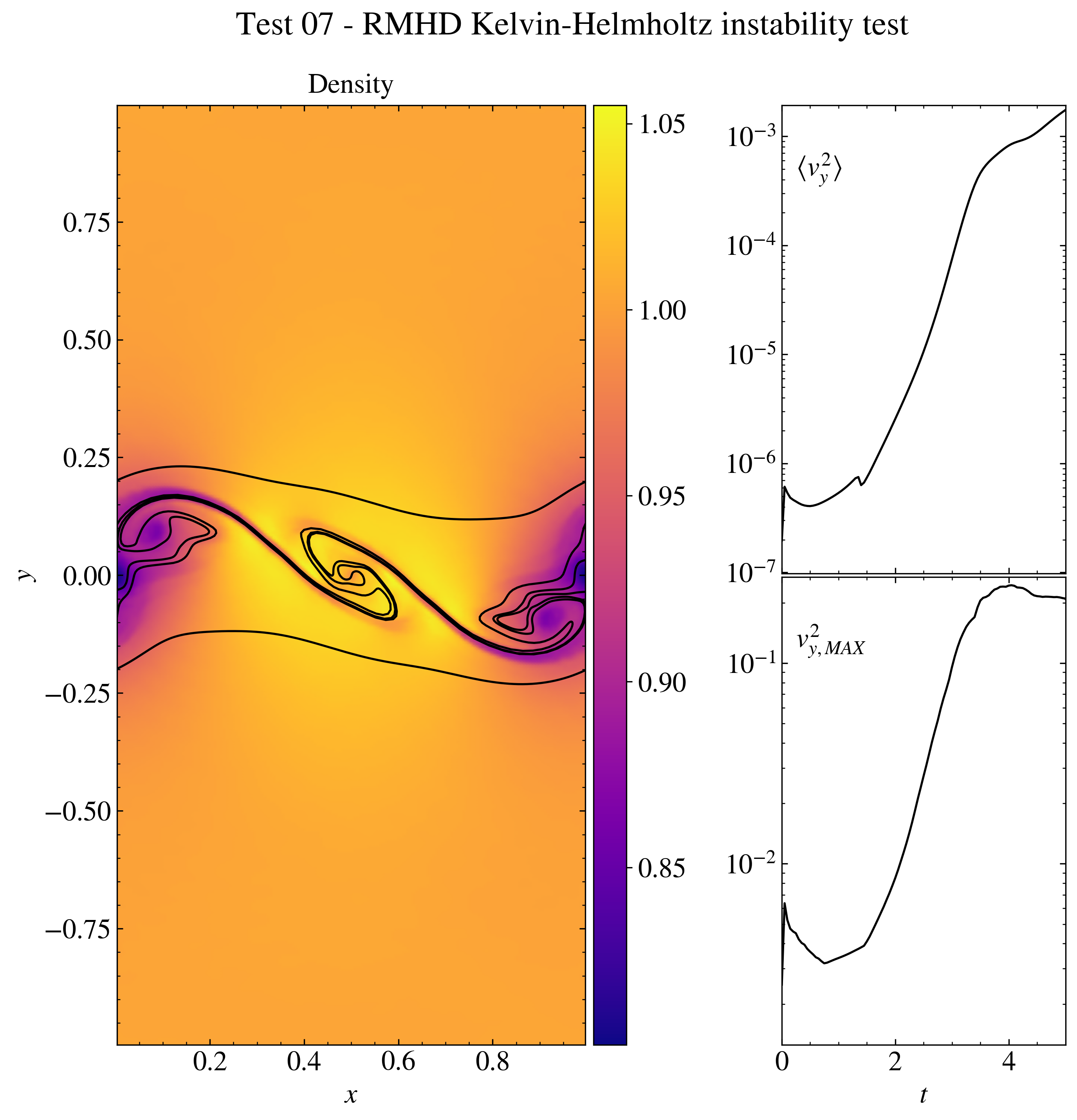
"""RMHD Kelvin-Helmholtz instability test.

This test shows how to plot a more complex figure with a customized number of
subplots and the insert of text inside the plots.

The data are the ones obtained from the PLUTO test problem
$PLUTO_DIR/Test_Problems/RMHD/KH (configuration 1).

The data is loaded into a pload object D and the Image class is created. The
create_axes method is used to form a collage of plots both elegant and useful.
The display method is used to plot the density in the main plot, while the plot
method, together with the text method, is used to show secondary plots of the
trasversal velocity as a function of time. The image is then saved and shown on
screen.

IMPORTANT: For the correct representation of the secondary plots, the analysis
parameter in the pluto.ini should be changed to 0.05.

"""

# Loading the relevant packages
import pyPLUTO

# Set the relative path to the data folder
data_path = pyPLUTO.find_example("RMHD/KH")

# Load data
Data = pyPLUTO.Load(path=data_path)

# Creating the image and the subplot axes (to have two secondary plots)
Image = pyPLUTO.Image(
    figsize=[10.5, 10],
    suptitle="Test 07 - RMHD Kelvin-Helmholtz instability test",
    nwin=7,
)
Image.create_axes(right=0.55)
Image.create_axes(nrow=2, hspace=[0.003], left=0.67)

# Plotting the data
Image.display(
    Data.rho,
    x1=Data.x1,
    x2=Data.x2,
    title="Density",
    aspect="equal",
    ax=0,
    shading="gouraud",
    xtitle=r"$x$",
    ytitle=r"$y$",
    cpos="right",
)

# Find and plot the field lines
lines = Data.find_fieldlines(
    Data.Bx1,
    Data.Bx2,
    x1=Data.x1,
    x2=Data.x2,
    y0=[0.0, 0.1, -0.1, 0.25, -0.25],
    x0=[0.5, 0.5, 0.5, 0.5, 0.5],
    order="RK45",
    maxstep=0.001,
    numsteps=10000,
)

for _, line in enumerate(lines):
    Image.plot(line[0], line[1], ax=0, c="k")

# Open the kh.dat file and store the variables
analysis = Data.read_file("kh.dat")

# Add text in the axes
Image.text(r"$\langle v_y^2\rangle$", ax=1, x=0.05)
Image.text(r"$v_{y, MAX}^2$", ax=2, x=0.05)

# Plot the velocity from the kh.dat file.
Image.plot(
    analysis["time"],
    analysis["vy2"],
    ax=1,
    c="k",
    yscale="log",
    xtickslabels=None,
)
Image.plot(
    analysis["time"],
    analysis["maxvy"],
    ax=2,
    c="k",
    yscale="log",
    xtitle=r"$t$",
)

# Saving the image and showing the plots
Image.savefig("test07_khi.png", script_relative=True)
# pyPLUTO.show()
 """RMHD Kelvin-Helmholtz instability test. This test shows how to plot a more complex figure with a customized number of subplots and the insert of text inside the plots. The data are the ones obtained from the PLUTO test problem $PLUTO_DIR/Test_Problems/RMHD/KH (configuration 1). The data is loaded into a pload object D and the Image class is created. The create_axes method is used to form a collage of plots both elegant and useful. The display method is used to plot the density in the main plot, while the plot method, together with the text method, is used to show secondary plots of the trasversal velocity as a function of time. The image is then saved and shown on screen. IMPORTANT: For the correct representation of the secondary plots, the analysis parameter in the pluto.ini should be changed to 0.05. """ # Loading the relevant packages import pyPLUTO # Set the relative path to the data folder data_path = pyPLUTO.find_example("RMHD/KH") # Load data Data = pyPLUTO.Load(path=data_path) # Creating the image and the subplot axes (to have two secondary plots) Image = pyPLUTO.Image( figsize=[10.5, 10], suptitle="Test 07 - RMHD Kelvin-Helmholtz instability test", nwin=7, ) Image.create_axes(right=0.55) Image.create_axes(nrow=2, hspace=[0.003], left=0.67) # Plotting the data Image.display( Data.rho, x1=Data.x1, x2=Data.x2, title="Density", aspect="equal", ax=0, shading="gouraud", xtitle=r"$x$", ytitle=r"$y$", cpos="right", ) # Find and plot the field lines lines = Data.find_fieldlines( Data.Bx1, Data.Bx2, x1=Data.x1, x2=Data.x2, y0=[0.0, 0.1, -0.1, 0.25, -0.25], x0=[0.5, 0.5, 0.5, 0.5, 0.5], order="RK45", maxstep=0.001, numsteps=10000, ) for _, line in enumerate(lines): Image.plot(line[0], line[1], ax=0, c="k") # Open the kh.dat file and store the variables analysis = Data.read_file("kh.dat") # Add text in the axes Image.text(r"$\langle v_y^2\rangle$", ax=1, x=0.05) Image.text(r"$v_{y, MAX}^2$", ax=2, x=0.05) # Plot the velocity from the kh.dat file. Image.plot( analysis["time"], analysis["vy2"], ax=1, c="k", yscale="log", xtickslabels=None, ) Image.plot( analysis["time"], analysis["maxvy"], ax=2, c="k", yscale="log", xtitle=r"$t$", ) # Saving the image and showing the plots Image.savefig("test07_khi.png", script_relative=True) # pyPLUTO.show()